
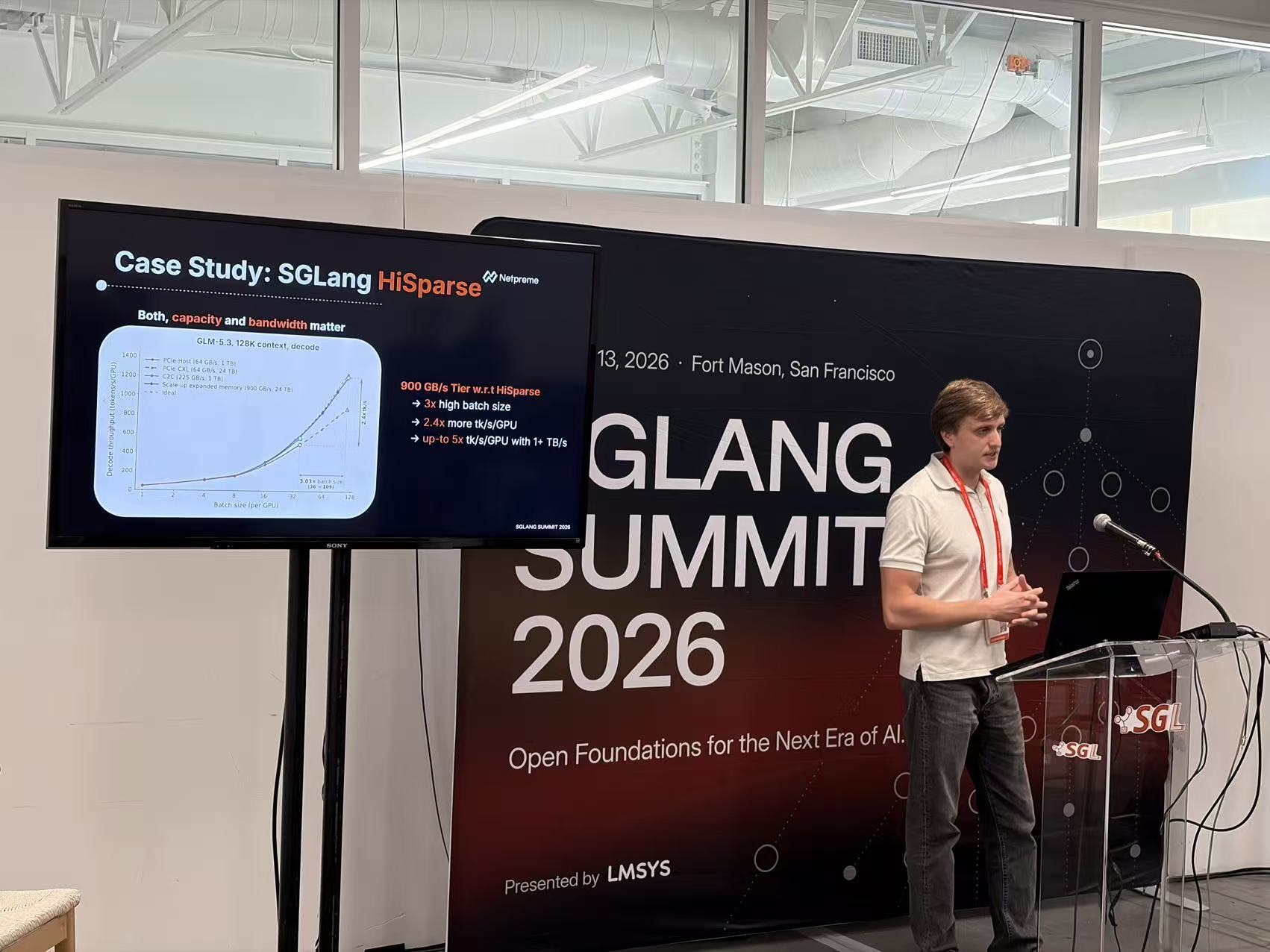
Longer contexts and larger batches put pressure on GPU memory, limiting how many requests an LLM serving system can handle. At SGLang Summit, Netpreme’s session explored how an external memory hierarchy can ease that constraint.
Nikita used SGLang HiSparse to show how memory tiering can work for LLM inference. HiSparse reads selected entries from the key-value (KV) cache during decoding but retains the full history. A small hot buffer stays in high-bandwidth memory (HBM), while the full cache can live in an external tier. The talk then examined the bandwidth and software needed to fetch selected entries efficiently.
Highlights
- HBM + external memory
Keep a hot KV buffer in HBM and the full history in an external tier.
- Top-k sparse attention
Read selected entries at each step. Retain the full cache for later selections.
- Data movement
Fetch primitives, attention kernels and memory management make the tier usable.
Why HBM capacity is difficult to scale
Nikita’s opening slides contrast hundreds of gigabytes of memory near compute with an illustrative target of 5 to 10 TB at HBM bandwidth.
That increase runs into limits in packaging, interconnect technology and manufacturing. Power, cooling and supply add further constraints. Even if a design is technically possible, its cost and reliability still need to hold up.
A memory hierarchy offers another way to add capacity. The design depends on which data must stay near the processor and how long the workload can wait for data stored farther away.
Models are changing how they use memory
Model architectures differ in how much state they retain and how they access it. Nikita discussed multi-head and grouped-query attention alongside multi-head latent attention, sparse attention and linear attention. He also pointed to Engrams and loop transformers as designs being explored.
These access patterns give hardware designers different options for placing data. Model design and memory design can develop together within physical and cost constraints.
The hierarchy in the talk leaves SRAM and HBM near compute and adds a larger external tier through a low-latency, high-bandwidth link. It calls for XPU-native unified memory and a memory-tiering library. Candidate uses include KV caches, sparse attention, Engrams and expert offloading.
Why HiSparse retains the full KV cache
During dense-attention decoding, a new token’s query is compared with keys across the retained context. The resulting attention weights determine how the corresponding values are combined.
In the top-k sparse-attention example, an indexer selects a subset of historical positions before attention uses their keys and values. Each decode step reads much less KV data than dense attention.
The selection can change with the next token, so an entry skipped now may be needed later. This approach still needs the full KV history. If all of it stays in HBM, storage capacity can limit both context length and the number of requests served at once.
How SGLang HiSparse uses KV cache offloading
In SGLang HiSparse, KV cache offloading keeps the full KV history in host memory while a small hot KV buffer remains in GPU HBM. Selected entries already in the buffer can be used locally; missing entries must be fetched from the external tier. In the DSA-style path shown here, the indexer key cache (K-index) also remains in HBM.
Nikita cited the HiSparse paper by Xie and colleagues, which reports up to 4.7× the peak generation throughput of its full-KV-in-HBM baseline on the long-context workloads it evaluated. Our study below examines how changing the external tier’s capacity and bandwidth affects performance.
In the Netpreme architecture shown in the talk, X-Mem™ holds the full KV cache. Prefill GPUs publish KV data to the pool, while decode GPUs keep their hot buffers in HBM and fetch missing selected entries over the scale-up fabric.
Capacity vs. bandwidth: the 128K-context study
Our GLM-5.3 study at 128K context compares four external-memory configurations. They vary the space available for the full KV cache and the bandwidth available to fetch selected entries during decode.
In our study, the modeled 900 GB/s tier supported roughly 3× the maximum batch size (36 → 109 requests per GPU) and 2.4× the peak decode throughput per GPU of the PCIe host-memory baseline. Peak throughput is compared at each configuration’s own peak batch size.
The C2C configuration raises bandwidth but keeps capacity at 1 TB, so the full-cache storage limit remains. PCIe-CXL adds capacity while holding bandwidth at 64 GB/s. It permits larger batches, but fetching their selected KV entries still limits throughput.
A fast memory tier still needs an efficient data path
To keep a high-bandwidth link busy, the system needs enough data transfers in flight while earlier requests complete. The amount of data needed is the bandwidth-delay product: bandwidth multiplied by latency.
Nikita’s example pairs terabytes-per-second bandwidth with microsecond-scale latency and accesses of about 800 bytes. Keeping enough of these small transfers in flight takes GPU resources to issue requests, track completion, stage results and coordinate dependencies.
Sparse attention also has to wait for the indexer’s selections before fetching missing entries. The implementation must handle data hazards and hide latency where dependencies allow.
If that fetch path is inefficient, much of the external tier’s bandwidth goes unused.
The software needed for memory tiering
Nikita outlined three parts of the software stack:
Data-movement primitives.
GPU-initiated DMA, scatter-gather operations and swap-in kernels move selected data. The slide includes DMA, TMA and cp.async as building blocks.
Workload-aware kernels.
Nikita described work on PoolSparse, combining HiSparse with a high-bandwidth external memory tier. He also discussed prefix-cache prefetchers; the appendix outlines GPU-initiated DMA and TMA-based fused, out-of-order attention.
Memory management.
An HBM-tier memory-management library would unite memory across the scale-up domain, including C2C-connected CPU memory, peer HBM and X-Mem. It would incorporate the movement primitives and kernels.
Kernel design has to account for both the model’s access pattern and the memory fabric.
Where model and memory design meet
The top-k sparse-attention approach in the talk gives memory-tiering designs a specific workload to support: a large retained KV history with a smaller set of entries used at each step. As HBM capacity remains difficult to scale, that difference creates room to design models and memory systems together.
There is still work to do on efficient HBM tiering. Our study shows how capacity and bandwidth affect the available batch size and peak throughput under the modeled assumptions. The data-movement primitives, kernels and memory-management library described in the talk address how to put that memory to use. Netpreme is exploring these components together as models’ access patterns evolve.